The Timebase — Mains 60 Hz

Every clock needs a reference — something that ticks at a known, steady rate, against which the counting logic accumulates seconds. In a wristwatch that reference is a quartz crystal; in a GPS-disciplined clock it is an atomic standard a continent away. The KABtronics Transistor Wall Clock has neither a crystal nor a real-time-clock chip nor a backup battery. Its reference is the 60 Hz alternating current coming out of the wall. The clock literally counts cycles of the power line: sixty cycles is one second, and a chain of dividers (Vol 4) turns that into the seconds, minutes, and hours on the display.

This is an old and honest choice. Mains-synchronous clocks — the buzzing kitchen clock, the synchronous wall clock of the mid-twentieth century — all worked this way, and for the same reason: the power company holds the line frequency astonishingly accurate over the long run, so a device that counts line cycles keeps better time, over a week, than most cheap crystals. The cost is that the clock has no memory of time: pull the plug, or suffer an outage, and it forgets the time completely and must be re-set by hand. There is no holdover.

What makes this volume worth a careful read is not the idea of counting the mains — that is simple — but the circuit that turns the soft, dirty, rectified line voltage into a crisp 60 Hz square wave the logic can count, and does so in a way that makes it impossible for electrical noise to make the clock run fast. That circuit, a pulser feeding a charge-and-compare network, is in effect a brick-wall low-pass filter, and it is the cleverest single idea in the whole design. We build up to it: first why the mains is a good timebase at all, then the power supply that feeds the board, then the extractor stage by stage, then the noise-rejection logic, and finally what accuracy you actually get.

6.1 Why count the mains?

A timebase is judged on two different timescales, and the mains scores very differently on each.

Long term, the mains is excellent. The North American grid is steered by the utilities so that the total number of cycles delivered over hours and days is held essentially exact. If the instantaneous frequency dips below 60 Hz during a heavy-load afternoon, the grid operators deliberately run it slightly fast later (overnight, say) so that the running cycle count catches back up. The control target is the accumulated count, not the instantaneous frequency, which is exactly what a clock cares about: a clock that counts cycles only needs the long-run count to be right. The practical consequence is that a mains-counting clock keeps time over days and weeks at least as well as an ordinary quartz movement, with no crystal to buy, trim, or age.¹

Short term, the mains wanders. The instantaneous line frequency is not a clean 60.000 Hz; it drifts a fraction of a percent up and down minute to minute as load comes and goes. A mains-counting clock therefore has visible short-term jitter — across a single minute it may be a hair fast or slow — but because the grid corrects the accumulated count, that jitter averages out and does not accumulate into a real error.

The trade-offs that come with the choice are the defining limitations of the design:

• No holdover. There is no crystal oscillator, no RTC chip, and no backup battery anywhere on the board. The instant power is removed — a pulled plug, a tripped breaker, a utility outage — the counters lose their state and the displayed time is gone. On restore the clock starts counting again from whatever the counters happen to power up to, and you must re-set the time by hand with the H (hours) and M (minutes) switches.
• It is a 60 Hz design. The prescaler that follows divides by sixty to make a one-second tick (§6.5). In a 50 Hz country the line delivers fifty cycles per second, so the same divider would run the clock 20 % fast (sixty counted “seconds” would elapse in fifty real ones). Using the clock on 50 Hz requires changing the prescaler’s divide ratio from ÷60 to ÷50 — a design change, not a switch setting. The KABtronics manual is a 60 Hz design.¹

So the bargain is plain: in exchange for outstanding long-term accuracy and a parts list with no precision frequency reference on it, you accept a clock that forgets the time when unplugged and that is wedded to the local line frequency.

6.2 The power supply

Before any of the logic can run, the board needs a steady low-voltage DC rail, and the same section that makes it also taps off the raw 60 Hz the timebase needs. Start with the DC supply.

A 9–12 V AC wall transformer — an ordinary plug-in “wall wart” with an AC (not DC) output — plugs into a two-position screw terminal at the edge of the board. Because the output is AC, the two leads are interchangeable; there is no polarity to observe at the terminal. The transformer’s secondary voltage is given only as the 9–12 V AC range; the exact figure is not specified in the manual and varies with the particular wall unit supplied.

On the board, the AC meets a full-wave bridge rectifier — four large rectifier diodes arranged in the classic diamond. On each half of the AC cycle, two of the four diodes conduct and steer current the same way into the rail, so the bridge folds both halves of the AC waveform into a single train of positive humps (pulsing DC at 120 Hz — twice the line frequency, because both halves are used). That pulsing DC is then smoothed by the supply’s one large energy store: a 6,800 µF electrolytic capacitor. The capacitor charges up on each hump and supplies the board through the troughs between humps, so the rail settles to a fairly steady DC.

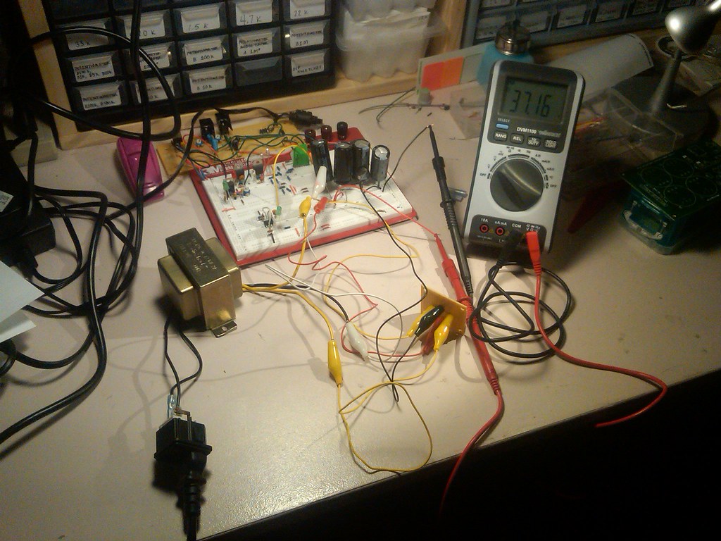
The manual’s bench check is to put a meter on that capacitor and look for about 13 V DC; it explicitly says “a few volts either way is OK,” since the exact figure depends on the transformer and on load. (Roughly, the capacitor charges toward the peak of the rectified AC — the peak of, say, a 9.5 V AC RMS secondary is about 13 V, less two diode drops — which is why ~13 V is the expected reading.) The whole board is a light load on this rail: the clock draws about 0.6 A at 9.5 V AC, roughly 5.7 W.¹

Two polarity cautions, and they are the only real hazards in this otherwise gentle build:

• The 6,800 µF electrolytic capacitor is polarized. Soldered in backwards it can heat up and, in the worst case, vent. Match its marked negative stripe to the board silkscreen.
• The four bridge diodes are polarized. Reversed, a diode in the bridge can short the transformer’s output and overheat the transformer. Match each diode’s banded (cathode) end to the silkscreen.

Beyond those two, the supply is friendly. The rail sits low enough — around 13 V — that the board is finger-safe: you can rest a fingertip on a transistor or resistor to feel whether it is running warm without any shock hazard, which is a genuinely useful troubleshooting tool on a board of a thousand parts (Vol 9). Nothing you can touch on the board is at line voltage; the mains stays sealed inside the wall transformer.

6.3 The 60 Hz extractor — overview

Here is the clever part, and the reason the power-supply section is not only a power supply.

The logic needs a clean digital clock: a square wave that is unambiguously HIGH or LOW, with exactly sixty crisp falling edges per second and not one extra. What the rectifier produces is the opposite of that — soft, rounded humps of pulsing DC riding on the rail, contaminated by whatever electrical noise the power line is carrying (motor brushes, switching loads, dimmers). You cannot feed that into a counter; you must first recover a clean 60 Hz timing signal from it.

The extractor does this in five stages, and the trick is that the middle of the chain deliberately throws away timing information in a way that makes noise harmless. Trace it:

bridge leg → 1st comparator (vs ~6 V) → 60 Hz pulse train → edge-detect pulser (discharges a small cap) → small cap ramps up through a resistor → 2nd comparator (vs ~6 V) → clean 60 Hz square wave → prescaler

Stage by stage:

6.3.1 Stage 1 — tap a bridge leg

Rather than tapping the smoothed DC rail (which has had its 60 Hz character filtered away by the big reservoir cap), the extractor taps one leg of the bridge rectifier — a point that still swings with the AC line at the line rate. This is the raw timing source: a waveform that rises and falls sixty times a second, locked to the mains.

6.3.2 Stage 2 — the first comparator squares it

That swinging leg voltage is fed to a comparator that compares it against a reference of about 6 V. (The comparator itself is the differential-pair circuit detailed in Vol 3 — reused here, not re-derived; the manual gives the reference only as approximately 6 V, and the exact figure is not specified.) Each time the leg voltage crosses the ~6 V threshold, the comparator snaps cleanly between its two output states. The soft analog hump becomes a hard digital 60 Hz pulse train — one pulse per line cycle, with sharp edges. So far this is the naive approach: square up the line and count its edges.

6.3.3 Stage 3 — the edge-detector and pulser

Now the clever turn. The 60 Hz pulse train is edge-detected: a small differentiating network responds only to the transitions of the pulse train, not its levels, and on each negative-going edge it fires a “pulser” — a transistor switch. When the pulser fires it briefly discharges a small capacitor, dumping its charge to (near) zero in an instant. So sixty times a second — once per line cycle — the pulser yanks this small capacitor down.

6.3.4 Stage 4 — the small cap ramps back up

Between pulser firings, that small capacitor charges back up through a resistor. The resistor–capacitor pair sets a charging rate, and that rate is chosen deliberately: it is just fast enough that the capacitor reaches the trip threshold roughly once per 60 Hz cycle, and no faster. The voltage on the cap therefore looks like a sawtooth: yanked to zero by the pulser, then ramping upward through the resistor, then yanked to zero again on the next line edge. (The specific small-cap and resistor values that set this rate are not given in the manual; only the behaviour — a ramp timed to the 60 Hz cycle — is described.)

6.3.5 Stage 5 — the second comparator makes the clean output

The ramping capacitor voltage is fed to a second comparator, again compared against about 6 V. When the ramp climbs past ~6 V the comparator snaps, producing the final clean 60 Hz square wave. Because the ramp can only reach threshold once per line cycle (Stage 4), this output is exactly one clean pulse per 60 Hz cycle — and that signal, sixty crisp edges a second, is what is handed to the prescaler (§6.5).

The reason for going to all this trouble — two comparators, a pulser, and a deliberately timed ramp, when a single comparator would seem to do the job — is the subject of the next section.

6.4 Why the elaborate path: a brick-wall noise filter

Imagine the naive timebase: tap the bridge leg, square it with one comparator, count the edges. It works perfectly on a clean line. But the power line is not clean — it carries spikes and bursts of electrical noise from every motor, switch, dimmer, and switching supply on the circuit. A naive comparator faithfully squares up every crossing of its threshold, noise included. A noise burst that briefly drives the leg voltage across ~6 V produces an extra edge, the counter logs an extra count, and the clock gains time — it runs fast, unpredictably, whenever the line is noisy. This is the failure mode the design is built to prevent.

The pulser-and-ramp stage defeats it by acting as a brick-wall low-pass filter with a cutoff of about 120 Hz. Here is the logic:

• The pulser fires — and resets the small cap to zero — on every negative-going edge the first comparator produces, including edges caused by noise.
• The second comparator can only assert its clean output when the small cap has had enough time to ramp all the way up to ~6 V, which by design takes one 60 Hz cycle.
• So if noise causes the first comparator to fire faster than 60 Hz — i.e., a second edge arrives before a full cycle has elapsed — the pulser discharges the cap again before it has finished ramping up. The ramp never reaches threshold, the second comparator never asserts, and no extra count is produced. The noise edge is simply swallowed.

In short: extra, too-soon edges reset the ramp instead of adding a count. The circuit will only emit an output pulse for edges spaced no closer than about one 60 Hz period apart, which is exactly the behaviour of a low-pass filter that rejects everything faster than ~120 Hz. Anything trying to clock the timebase faster than the line rate is filtered out.²

There is a complementary reason this is safe, having to do with the shape of real line noise. Genuine electrical noise on the mains comes in short bursts — spikes far shorter than the 16.7 ms of a single 60 Hz cycle. The worst such a burst can do is fire the pulser a little early within a cycle, which merely shortens that one ramp before the legitimate next edge would have reset it anyway. It cannot manufacture a whole extra cycle’s worth of ramp-and-trip, so it cannot add a count. Slow noise that genuinely persisted for a full cycle would be a different matter — but real line noise does not look like that.

Contrast the two designs squarely:

• Naive single comparator: every noise crossing = an extra edge = an extra count → the clock gains time on a noisy line. The error accumulates and is one-directional (always fast).
• Pulser + ramp + second comparator: noise edges only reset the ramp; they cannot create a trip the ramp hasn’t earned → the clock ignores the noise and keeps counting at the true line rate.

That asymmetry — that the worst a fast noise edge can do is reset a ramp, never add a count — is why the clock does not run fast in an electrically dirty room. It is a remarkable amount of robustness for a handful of discrete parts, and it is the single design idea most worth carrying away from this volume.

6.5 Feeding the prescaler

The extractor’s job ends with that clean 60 Hz square wave; the counting logic takes it from there. The first thing the logic does is divide it down to a one-second tick, and the arithmetic is exactly what you would expect from “sixty cycles per second”:

$$60 \text{ Hz} ;\xrightarrow{;\div 10;}; 6 \text{ Hz} ;\xrightarrow{;\div 6;}; 1 \text{ Hz}$$

A ÷10 stage takes the 60 Hz down to 6 Hz, and a ÷6 stage takes that to 1 Hz — one clean pulse per second. Sixty cycles in, one tick out: $60 / (10 \times 6) = 1$. That 1 Hz tick is the heartbeat the rest of the clock counts — into seconds (÷10, ÷6), minutes (÷10, ÷6), and hours (÷12) — and the full divide chain, including how each ÷10, ÷6, and ÷12 stage is built from toggle flip-flops and steering logic, is the subject of Vol 4. This volume’s responsibility ends at the hand-off: a clean, noise-immune 60 Hz square wave delivered to the prescaler’s input.

(This is also where the 50 Hz problem of §6.1 lives: on a 50 Hz line you would need the prescaler to divide by fifty rather than sixty — for example ÷10 then ÷5 — to recover a true 1 Hz. With the 60 Hz divider unchanged, a 50 Hz line yields only $50/60 = 0.833$ of a tick per second and the clock runs slow; viewed the other way, the clock counts 60 of its “seconds” in 50 real ones and so runs fast against the wall. Either way it is wrong by the 50:60 ratio, which is why the divider — not a setting — must change.)

6.6 Accuracy in practice

Put the pieces together and the practical behaviour of this timebase is easy to summarize.

• Long term: excellent. Because the utility steers the grid to hold the accumulated cycle count essentially exact (§6.1), a clock that counts those cycles keeps very good time over days and weeks — comparable to or better than an untrimmed quartz movement, and with no crystal anywhere in the bill of materials.
• Short term: small jitter, self-correcting. The instantaneous line frequency wanders a fraction of a percent with load, so over any single minute the clock may run a hair fast or slow. That jitter does not accumulate, because the grid’s correction pulls the long-run count back to true. You will not see it on the display; you would see it only on an instrument watching the line.
• Noise: rejected. The brick-wall filter of §6.4 means a noisy power line does not make the clock gain time — the failure mode of a naive design is engineered out.
• Holdover: none. No crystal, no RTC, no battery. Power loss erases the time, and the clock must be re-set by hand on restore (§6.1). This is the one genuine inconvenience of the design, and it is inherent to a mains-counted clock with no backup store.

For a clock whose entire reason to exist is to make digital logic visible (Vol 1), the mains timebase is the right match: it adds no opaque precision part — no crystal can, no RTC chip — and instead derives the reference from the wall through a circuit you can probe node by node on a scope, watching the soft hump become a pulse train, become a sawtooth, become a clean square wave. The timebase is as transparent as the rest of the clock.

Source hint: license-clean image via the Photo Helper — Wikimedia Commons / Openverse search for "AC adapter wall transformer", "bridge rectifier diodes", or "electrolytic capacitor"; credit verbatim in the caption. Reference-only web image acceptable if no CC-clean image is found.

6.7 References

• KABtronics Transistor Wall Clock Kit — assembly manual (Theory of Operation, Circuit Description) and 15-page schematic, in 02-inputs/LED_Transistor_Clock/. Vendor: http://www.transistorclock.com.
• Cross-references: Vol 3 (the differential-pair comparator), Vol 4 (the prescaler and the full ÷10 / ÷6 / ÷12 divide chain), Vol 1 (the system overview and the signal chain).

Footnotes

1. Transistor Clock Assembly Manual, KABtronics (transistorclock.com), Theory of Operation and Circuit Description sections. Source for: the 9–12 V AC wall-transformer input to a two-position screw terminal; the four-diode bridge rectifier; the 6,800 µF reservoir capacitor checked for ~13 V DC (“a few volts either way is OK”); the ~0.6 A / ~5.7 W (at 9.5 V AC) board consumption; the polarity cautions on the electrolytic capacitor and the bridge diodes; the finger-safe low-voltage rail; the no-crystal / no-RTC / no-battery, mains-counted 60 Hz timebase and the loss of time on power-off; and the 60 Hz design (a 50 Hz line requires a different prescaler divide ratio). Exact transformer secondary voltage (beyond “9–12 V AC”), exact comparator reference voltages (beyond “~6 V”), and the small-cap / resistor values in the extractor are not specified in the manual and are not invented here. ↩ ↩² ↩³

2. The brick-wall ~120 Hz low-pass interpretation of the pulser-and-ramp stage follows the manual’s Theory of Operation: the pulser discharges the small capacitor on each line edge, and the capacitor’s charge rate through its resistor is set so the second comparator can trip only once per 60 Hz cycle, so an edge arriving faster than the line rate resets the ramp rather than producing a count. The comparator circuit itself (a differential pair) is treated in Vol 3; the divide chain that consumes the clean 60 Hz is Vol 4. ↩